Intro to DoWhy#
import kagglehub

# Download latest version
path = kagglehub.dataset_download("tbyrnes/advertising")

print("Path to dataset files:", path)
Path to dataset files: /Users/hunter.lybbert/.cache/kagglehub/datasets/tbyrnes/advertising/versions/1
import pandas as pd
raw_df = pd.read_csv("/Users/hunter.lybbert/.cache/kagglehub/datasets/tbyrnes/advertising/versions/1/advertising.csv")
raw_df.head()
| Daily Time Spent on Site | Age | Area Income | Daily Internet Usage | Ad Topic Line | City | Male | Country | Timestamp | Clicked on Ad | |
|---|---|---|---|---|---|---|---|---|---|---|
| 0 | 68.95 | 35 | 61833.90 | 256.09 | Cloned 5thgeneration orchestration | Wrightburgh | 0 | Tunisia | 2016-03-27 00:53:11 | 0 |
| 1 | 80.23 | 31 | 68441.85 | 193.77 | Monitored national standardization | West Jodi | 1 | Nauru | 2016-04-04 01:39:02 | 0 |
| 2 | 69.47 | 26 | 59785.94 | 236.50 | Organic bottom-line service-desk | Davidton | 0 | San Marino | 2016-03-13 20:35:42 | 0 |
| 3 | 74.15 | 29 | 54806.18 | 245.89 | Triple-buffered reciprocal time-frame | West Terrifurt | 1 | Italy | 2016-01-10 02:31:19 | 0 |
| 4 | 68.37 | 35 | 73889.99 | 225.58 | Robust logistical utilization | South Manuel | 0 | Iceland | 2016-06-03 03:36:18 | 0 |
raw_df.rename(columns=lambda x:x.replace(' ', '_').lower(),inplace=True)
raw_df.columns
Index(['daily_time_spent_on_site', 'age', 'area_income',
       'daily_internet_usage', 'ad_topic_line', 'city', 'male', 'country',
       'timestamp', 'clicked_on_ad'],
      dtype='str')
df = raw_df.copy(deep=True)
df.timestamp = pd.to_datetime(df.timestamp)
df["day_of_week"] = df["timestamp"].dt.dayofweek
df["hour"] = df["timestamp"].dt.hour
df["month"] = df["timestamp"].dt.month
df.drop(columns=["timestamp"], inplace=True)
df.dtypes
daily_time_spent_on_site    float64
age                           int64
area_income                 float64
daily_internet_usage        float64
ad_topic_line                   str
city                            str
male                          int64
country                         str
clicked_on_ad                 int64
day_of_week                   int32
hour                          int32
month                         int32
dtype: object
# age -> daily_time_spent_on_site;
# age -> daily_internet_usage;
# male -> daily_internet_usage;
# male -> daily_time_spent_on_site;
# daily_time_spent_on_site -> timestamp;
# daily_internet_usage -> timestamp;
# daily_time_spent_on_site -> clicked_on_ad;
# daily_internet_usage -> clicked_on_ad;
# country -> area_income -> clicked_on_ad;
# country -> daily_internet_usage;
# area_income -> daily_time_spent_on_site;
# area_income -> daily_internet_usage;
# area_income -> clicked_on_ad;
# city -> country -> area_income -> clicked_on_ad;
# city -> area_income;

# 'daily_internet_usage',
# 'ad_topic_line',
# 'city',
# 'male',
# 'country',
# 'timestamp',
# 'clicked_on_ad'
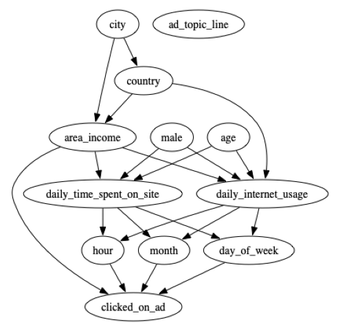
causal_graph = """
digraph {
daily_time_spent_on_site;
age;
area_income;
daily_internet_usage;
ad_topic_line;
city;
male;
country;
day_of_week;
hour;
month;
clicked_on_ad;
age -> daily_time_spent_on_site;
age -> daily_internet_usage;
male -> daily_internet_usage;
male -> daily_time_spent_on_site;
daily_time_spent_on_site -> day_of_week;
daily_internet_usage -> day_of_week;
daily_time_spent_on_site -> month;
daily_internet_usage -> month;
daily_time_spent_on_site -> hour;
daily_internet_usage -> hour;
country -> area_income -> clicked_on_ad;
country -> daily_internet_usage;
area_income -> daily_time_spent_on_site;
area_income -> daily_internet_usage;
area_income -> clicked_on_ad;
city -> country -> area_income -> clicked_on_ad;
city -> area_income;
day_of_week -> clicked_on_ad;
hour -> clicked_on_ad;
month -> clicked_on_ad;
}
"""
# ad_topic_line -> clicked_on_ad;
from dowhy import CausalModel
model = CausalModel(
    data=df,
    graph=causal_graph.replace("\n", " "),
    treatment="hour",
    outcome="clicked_on_ad",
)
model.view_model()
# df.ad_topic_line.head(25)
0                Cloned 5thgeneration orchestration
1                Monitored national standardization
2                  Organic bottom-line service-desk
3             Triple-buffered reciprocal time-frame
4                     Robust logistical utilization
5                   Sharable client-driven software
6                        Enhanced dedicated support
7                          Reactive local challenge
8                    Configurable coherent function
9                Mandatory homogeneous architecture
10                   Centralized neutral neural-net
11    Team-oriented grid-enabled Local Area Network
12            Centralized content-based focus group
13                 Synergistic fresh-thinking array
14                    Grass-roots coherent extranet
15               Persistent demand-driven interface
16               Customizable multi-tasking website
17                       Intuitive dynamic attitude
18     Grass-roots solution-oriented conglomeration
19                       Advanced 24/7 productivity
20            Object-based reciprocal knowledgebase
21                Streamlined non-volatile analyzer
22            Mandatory disintermediate utilization
23               Future-proofed methodical protocol
24                    Exclusive neutral parallelism
Name: ad_topic_line, dtype: str
# model = CausalModel(
#     data=df,
#     graph=causal_graph.replace("\n", " "),
#     treatment="timestamp",
#     outcome="clicked_on_ad",
# )
# model.view_model()
estimands = model.identify_effect()
print(estimands)
Estimand type: EstimandType.NONPARAMETRIC_ATE

### Estimand : 1
Estimand name: backdoor
Estimand expression:
   d
───────(E[clicked_on_ad|daily_internet_usage,daily_time_spent_on_site])
d[hour]
Estimand assumption 1, Unconfoundedness: If U→{hour} and U→clicked_on_ad then P(clicked_on_ad|hour,daily_internet_usage,daily_time_spent_on_site,U) = P(clicked_on_ad|hour,daily_internet_usage,daily_time_spent_on_site)

### Estimand : 2
Estimand name: iv
No such variable(s) found!

### Estimand : 3
Estimand name: frontdoor
No such variable(s) found!

### Estimand : 4
Estimand name: general_adjustment
Estimand expression:
   d
───────(E[clicked_on_ad|daily_internet_usage,daily_time_spent_on_site])
d[hour]
Estimand assumption 1, Unconfoundedness: If U→{hour} and U→clicked_on_ad then P(clicked_on_ad|hour,daily_internet_usage,daily_time_spent_on_site,U) = P(clicked_on_ad|hour,daily_internet_usage,daily_time_spent_on_site)
estimate = model.estimate_effect(
    identified_estimand=estimands,
    method_name="backdoor.linear_regression",
    # method_name="backdoor.econml.dml.CausalForestDML",
    confidence_intervals=True,
    test_significance=True,
    # method_params={
    #     "init_params": {
    #         "n_estimators": 100,
    #         "random_state": 42
    #     }
    # }
)

print(f'Estimate of causal effect: {estimate}')
Estimate of causal effect: *** Causal Estimate ***

## Identified estimand
Estimand type: EstimandType.NONPARAMETRIC_ATE

### Estimand : 1
Estimand name: backdoor
Estimand expression:
   d
───────(E[clicked_on_ad|daily_internet_usage,daily_time_spent_on_site])
d[hour]
Estimand assumption 1, Unconfoundedness: If U→{hour} and U→clicked_on_ad then P(clicked_on_ad|hour,daily_internet_usage,daily_time_spent_on_site,U) = P(clicked_on_ad|hour,daily_internet_usage,daily_time_spent_on_site)

## Realized estimand
b: clicked_on_ad~hour+daily_internet_usage+daily_time_spent_on_site+hour*day_of_week+hour*month
Target units:

## Estimate
Mean value: -0.00046934978493284873
p-value: [0.74907975]
95.0% confidence interval: (np.float64(-0.002546200086192607), np.float64(0.0018146626893807971))
### Conditional Estimates
__categorical__day_of_week  __categorical__month
(-0.001, 1.0]               (0.999, 2.0]           -0.000541
                            (2.0, 3.0]             -0.000529
                            (3.0, 4.0]             -0.000526
                            (4.0, 6.0]             -0.000513
                            (6.0, 7.0]             -0.000502
(1.0, 2.0]                  (0.999, 2.0]           -0.000507
                            (2.0, 3.0]             -0.000498
                            (3.0, 4.0]             -0.000491
                            (4.0, 6.0]             -0.000480
                            (6.0, 7.0]             -0.000470
(2.0, 4.0]                  (0.999, 2.0]           -0.000475
                            (2.0, 3.0]             -0.000467
                            (3.0, 4.0]             -0.000457
                            (4.0, 6.0]             -0.000448
                            (6.0, 7.0]             -0.000438
(4.0, 5.0]                  (0.999, 2.0]           -0.000445
                            (2.0, 3.0]             -0.000434
                            (3.0, 4.0]             -0.000427
                            (4.0, 6.0]             -0.000415
                            (6.0, 7.0]             -0.000406
(5.0, 6.0]                  (0.999, 2.0]           -0.000422
                            (2.0, 3.0]             -0.000412
                            (3.0, 4.0]             -0.000405
                            (4.0, 6.0]             -0.000395
                            (6.0, 7.0]             -0.000384
dtype: float64
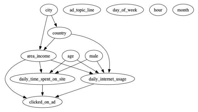
causal_graph_updated = """
digraph {
daily_time_spent_on_site;
age;
area_income;
daily_internet_usage;
ad_topic_line;
city;
male;
country;
day_of_week;
hour;
month;
clicked_on_ad;
age -> daily_time_spent_on_site;
age -> daily_internet_usage;
male -> daily_internet_usage;
male -> daily_time_spent_on_site;
daily_time_spent_on_site -> clicked_on_ad;
daily_internet_usage -> clicked_on_ad;
country -> area_income -> clicked_on_ad;
country -> daily_internet_usage;
area_income -> daily_time_spent_on_site;
area_income -> daily_internet_usage;
area_income -> clicked_on_ad;
city -> country -> area_income -> clicked_on_ad;
city -> area_income;
}
"""
# ad_topic_line -> clicked_on_ad;

model_updated = CausalModel(
    data=df,
    graph=causal_graph_updated.replace("\n", " "),
    treatment="daily_internet_usage",
    outcome="clicked_on_ad",
)
model_updated.view_model()
estimands_updated = model_updated.identify_effect()
print(estimands_updated)
Estimand type: EstimandType.NONPARAMETRIC_ATE

### Estimand : 1
Estimand name: backdoor
Estimand expression:
           d
───────────────────────(E[clicked_on_ad|area_income,daily_time_spent_on_site])
d[daily_internet_usage]
Estimand assumption 1, Unconfoundedness: If U→{daily_internet_usage} and U→clicked_on_ad then P(clicked_on_ad|daily_internet_usage,area_income,daily_time_spent_on_site,U) = P(clicked_on_ad|daily_internet_usage,area_income,daily_time_spent_on_site)

### Estimand : 2
Estimand name: iv
No such variable(s) found!

### Estimand : 3
Estimand name: frontdoor
No such variable(s) found!

### Estimand : 4
Estimand name: general_adjustment
Estimand expression:
           d
───────────────────────(E[clicked_on_ad|age,area_income,male])
d[daily_internet_usage]
Estimand assumption 1, Unconfoundedness: If U→{daily_internet_usage} and U→clicked_on_ad then P(clicked_on_ad|daily_internet_usage,age,area_income,male,U) = P(clicked_on_ad|daily_internet_usage,age,area_income,male)
estimate = model_updated.estimate_effect(
    identified_estimand=estimands_updated,
    method_name="backdoor.linear_regression",
    # method_name="backdoor.econml.dml.CausalForestDML",
    confidence_intervals=True,
    test_significance=True,
    # method_params={
    #     "init_params": {
    #         "n_estimators": 100,
    #         "random_state": 42
    #     }
    # }
)

print(f'Estimate of causal effect: {estimate}')
Estimate of causal effect: *** Causal Estimate ***

## Identified estimand
Estimand type: EstimandType.NONPARAMETRIC_ATE

### Estimand : 1
Estimand name: backdoor
Estimand expression:
           d
───────────────────────(E[clicked_on_ad|area_income,daily_time_spent_on_site])
d[daily_internet_usage]
Estimand assumption 1, Unconfoundedness: If U→{daily_internet_usage} and U→clicked_on_ad then P(clicked_on_ad|daily_internet_usage,area_income,daily_time_spent_on_site,U) = P(clicked_on_ad|daily_internet_usage,area_income,daily_time_spent_on_site)

## Realized estimand
b: clicked_on_ad~daily_internet_usage+area_income+daily_time_spent_on_site+daily_internet_usage*daily_time_spent_on_site
Target units:

## Estimate
Mean value: -0.005637221868382003
p-value: [0.41300316]
95.0% confidence interval: (np.float64(-0.006068843513229671), np.float64(-0.005152822316435213))
### Conditional Estimates
__categorical__daily_time_spent_on_site
(32.599000000000004, 47.23]   -0.003223
(47.23, 62.26]                -0.004660
(62.26, 72.952]               -0.005953
(72.952, 79.982]              -0.006809
(79.982, 91.43]               -0.007554
dtype: float64
model_updated_2 = CausalModel(
    data=df,
    graph=causal_graph_updated.replace("\n", " "),
    treatment="daily_time_spent_on_site",
    outcome="clicked_on_ad",
)

estimands_updated = model_updated_2.identify_effect()
print(estimands_updated)

estimate = model_updated_2.estimate_effect(
    identified_estimand=estimands_updated,
    method_name="backdoor.linear_regression",
    # method_name="backdoor.econml.dml.CausalForestDML",
    confidence_intervals=True,
    test_significance=True,
    # method_params={
    #     "init_params": {
    #         "n_estimators": 100,
    #         "random_state": 42
    #     }
    # }
)

print(f'Estimate of causal effect: {estimate}')
Estimand type: EstimandType.NONPARAMETRIC_ATE

### Estimand : 1
Estimand name: backdoor
Estimand expression:
            d
──────────────────────────(E[clicked_on_ad|area_income,daily_internet_usage])
d[dailyₜᵢₘₑ ₛₚₑₙₜ ₒₙ ₛᵢₜₑ]
Estimand assumption 1, Unconfoundedness: If U→{daily_time_spent_on_site} and U→clicked_on_ad then P(clicked_on_ad|daily_time_spent_on_site,area_income,daily_internet_usage,U) = P(clicked_on_ad|daily_time_spent_on_site,area_income,daily_internet_usage)

### Estimand : 2
Estimand name: iv
No such variable(s) found!

### Estimand : 3
Estimand name: frontdoor
No such variable(s) found!

### Estimand : 4
Estimand name: general_adjustment
Estimand expression:
            d
──────────────────────────(E[clicked_on_ad|age,area_income,male])
d[dailyₜᵢₘₑ ₛₚₑₙₜ ₒₙ ₛᵢₜₑ]
Estimand assumption 1, Unconfoundedness: If U→{daily_time_spent_on_site} and U→clicked_on_ad then P(clicked_on_ad|daily_time_spent_on_site,age,area_income,male,U) = P(clicked_on_ad|daily_time_spent_on_site,age,area_income,male)

Estimate of causal effect: *** Causal Estimate ***

## Identified estimand
Estimand type: EstimandType.NONPARAMETRIC_ATE

### Estimand : 1
Estimand name: backdoor
Estimand expression:
            d
──────────────────────────(E[clicked_on_ad|area_income,daily_internet_usage])
d[dailyₜᵢₘₑ ₛₚₑₙₜ ₒₙ ₛᵢₜₑ]
Estimand assumption 1, Unconfoundedness: If U→{daily_time_spent_on_site} and U→clicked_on_ad then P(clicked_on_ad|daily_time_spent_on_site,area_income,daily_internet_usage,U) = P(clicked_on_ad|daily_time_spent_on_site,area_income,daily_internet_usage)

## Realized estimand
b: clicked_on_ad~daily_time_spent_on_site+area_income+daily_internet_usage+daily_time_spent_on_site*daily_internet_usage
Target units:

## Estimate
Mean value: -0.01407526806184456
p-value: [0.16069722]
95.0% confidence interval: (np.float64(-0.015233356611323856), np.float64(-0.012781125853657649))
### Conditional Estimates
__categorical__daily_internet_usage
(104.779, 132.366]   -0.008043
(132.366, 163.44]    -0.010821
(163.44, 198.948]    -0.014298
(198.948, 224.836]   -0.017275
(224.836, 269.96]    -0.019939
dtype: float64
Start here by refuting the estimates that you developed, rework naming from the top so it is clear which models, graphs, and estimates/estimands are from which version of the modeling setup.
# From Claude:
# 1. Placebo treatment refuter — randomizes the treatment; a real effect should vanish.
#    Most diagnostic given your CI/p-value disagreement: if a *placebo* treatment also
#    produces a "significant"-looking estimate under this same estimator, the significance
#    test itself is unreliable, not just this particular result.
res_placebo = model_updated.refute_estimate(
    estimands_updated,
    estimate,
    method_name="placebo_treatment_refuter",
    placebo_type="permute",
    num_simulations=100,
)
print(res_placebo)

# 2. Random common cause — adds an independent random covariate as a confounder.
#    A robust estimate should barely move.
res_random_cc = model_updated.refute_estimate(
    estimands_updated,
    estimate,
    method_name="random_common_cause",
    num_simulations=100,
)
print(res_random_cc)

# 3. Data subset refuter — refits on random subsets of the data.
#    A stable effect should stay close to the full-sample estimate across subsets.
res_subset = model_updated.refute_estimate(
    estimands_updated,
    estimate,
    method_name="data_subset_refuter",
    subset_fraction=0.8,
    num_simulations=100,
)
print(res_subset)
  Cell In[36], line 1
    From Claude:
         ^
SyntaxError: invalid syntax